Quantifying Results: p-Value
In addition to computing the range of likely results from the model, statisticians also typically provide a quantification of the consistency between the observed result and the expectations based on the model. This quantification is referred to as a \(p\)-value (the \(p\) stands for probability).
To compute a \(p\)-value, you count the number of results that are at least as extreme as the observed result, and divide this by the total number of results.
\[ p = \frac{\mathrm{number~of~results~at~least~as~extreme~as~observed~result}}{\mathrm{total~number~of~simulated~results}} \]
This value is then reported as a decimal value. It quantifies the probability of observing a result at least as extreme as the observed result under the hypothesized model. It is often interpreted as the likelihood of the observed result given the hypothesized model.
To illustrate this, we will re-examine simulation results from the Sleep Deprivation study. Recall in that activity, the observed data had a difference in means of 15.9. Below is a plot of 100 differences in means simulated under the “no-effect”” model. A vertical line is shown at the observed difference of 15.9.
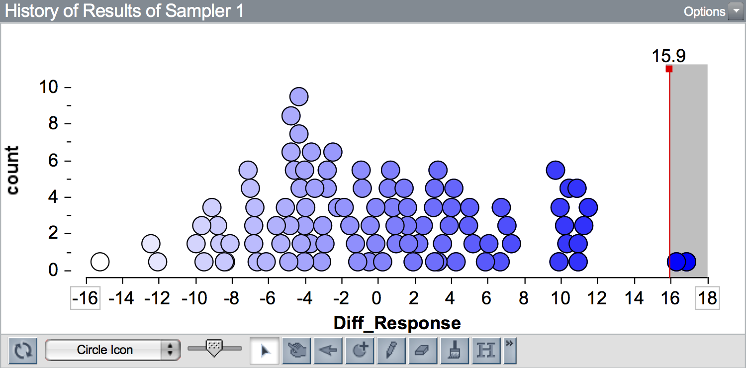
Since 15.9 is to the right of 0 (i.e., it is on the right-hand side of the plot) results that are more extreme than the observed result are to the right of 15.9. (If the observed result was to the left of 0, more extreme results would be those more negative than the observed result.) Here there are two simulated results out of 100 that are at least as extreme as 15.9 (\(\geq 15.9\)). We would report the \(p\)-value as 0.02.
Adjustment for Simulation Results
In simulation studies, we make one small adjustment to the \(p\)-value computation; we add 1 to both the numerator and denominator:
\[ p = \frac{\mathrm{number~of~results~more~extreme~than~observed} + 1}{\mathrm{total~number~of~simulated~results} + 1} \]
This adjustment assures that we never get a \(p\)-value of 0. Consider the \(p\)-value if our observed result would have been 18 (instead of 15.9). There are 0 results that are at least as extreme as 18 (\(\geq 18\)). The problem is that we only ran 100 trials of the simulation. If we had run this simulation for all possible randomizations of the data (i.e., infinitely many times), we would have seen results \(\geq 18\). So, to report a \(p\)-value of 0 is misleading. The \(p\)-value we report should be,
\[ p = \frac{0 + 1}{100 + 1} = 0.0099 \]
After the adjustment, the \(p\)-value is still quite small, indicating that had we seen an observed result of 18, we would say that it is not consistent with the model of “no-effect”. In fact it is in the outer 0.01 (1%) of the results simulated from the hypothesized model.
Going back to the \(p\)-value computed from the observed value of 15.9,
\[ p = \frac{2 + 1}{100 + 1} = 0.0297 \]
We can interpret the \(p\)-value of 0.030 as indicating that the observed difference of 15.9 is in the outer 0.03 (3%) of results simulated from the hypothesized model. It is quite unlikely that we would see a result as extreme as 15.9, or more extreme, under the hypothesized model of “no effect”. Thus, this observation is not consistent with our expectations based on the hypothesized model.
p-Values as Evidence
Large \(p\)-values indicate that the observed data are more consistent with the results from the model, while small \(p\)-values indicate that the observed data are not very consistent with the results from the model. As researchers, our goal is often to then translate this quantitative evidence into support for or against the hypothesized model. For example, in the Sleep Deprivation study, we obtained a \(p\)-value of 0.03. This suggests a low degree of consistency between the observed data (our empirical evidence) and the hypothesized model of “no effect”.
The broader scientific question about whether sleep deprivation has a harmful effect on learning, however is difficult to ascertain from a \(p\)-value. There are no hard-and-fast rules for gauging how strong the evidence is against the hypothesized model because what counts as evidence in one scientific discipline or context may not count in another scientific discipline or context. And, even if there were rules about the degree of evidence needed, you would still need to evaluate other criteria such as internal and external validity evidence, and sample size. Even then, the results from a single study are not typically convincing enough for most scientists to draw definitive conclusions. It is only through consistent findings that emerge from multiple studies (which may take decades) that we may have convincing evidence about the answer to the broader scientific question.
Six Principles about p-Values
Because they are so ubiquitous in the research literature for any field, and because they are often mis-interpreted (even by PhDs, researchers, and math teachers) it is important to be aware of what a \(p\)-value tells you, and more importantly, what it doesn’t tell you. To this end, the American Statistical Association released a statement on \(p\)-values in which it listed six principles:4
- Principle 1: \(P\)-values can indicate how incompatible the data are with a specified statistical model.
- Principle 2: \(P\)-values do not measure the probability that the studied hypothesis is true, or the probability that the data were produced by random chance alone.
- Principle 3: Scientific conclusions and business or policy decisions should not be based only on whether a \(p\)-value passes a specific threshold.
- Principle 4: Proper inference requires full reporting and transparency.
- Principle 5: A \(p\)-value does not measure the size of an effect or the importance of a result.
- Principle 6: By itself, a \(p\)-value does not provide a good measure of evidence regarding a model or hypothesis.
Guidelines for interpreting p-Values
Even though you should never interpret \(p\)-values against a fixed criteria, a good benchmark to help get a feel for how to interpret them in terms of consistency with a hypothesis are as follows:
- A \(p\)-value of less than .03 is often seen as an indication that the observed data is not consistent with the hypothesis.
- A \(p\)-value greater .03 but less than .08 is often seen as an indication that the observed data is only slightly consistent with the hypothesis.
- A \(p\)-value greater than .08 is often seen as an indication that that is relatively consistent with the hypothesis.
What do we do when we have seen observed some data that is not consistent with a hypothesis that we considered? We can not ignore the fact that we have observed something from the real world. One possibility is that the hypothesis is correct, but something else affected the study that we did not account for in our analysis. Another possibility is that the hypothesis is not correct. Scientists often focus on this second possibility, and interpret \(p\)-values in terms of how strongly they support the claim that the hypothesis is not correct. Re-interpreting the benchmark \(p\)-values above in this way suggests:
- A \(p\)-value of less than .03 is often seen as strong evidence against a hypothesis.
- A \(p\)-value greater .03 but less than .08 is often seen as indeterminate evidence against a hypothesis.
- A \(p\)-value greater than .08 is often seen as very weak evidence against a hypothesis.
While you can use these benchmarks to help you get a feel for interpreting \(p\)-values, be sure to remember Principle #3 from above – Scientific conclusions and business or policy decisions should not be based only on whether a \(p\)-value passes a specific threshold. These thresholds are only a guideline, but they are no substitute for being thoughtful and considering other aspects of the study and associated theories.
Yaddanapudi (2016) published a paper in the Journal of Anaesthesiology, Clinical Pharmacology in which she explains each of these six principles for practicing physician-scientists using an example of treatment efficacy for a drug.↩︎